Solving Kepler’s Equation

Warning: The routines below, that has B2 perturbations have a bug. For some values the orbit is reflected through the origin. I will put a fix here as soon as I find one. For the time being, please do not use drift_shep_pert() routines!

Warning2: This is simply a copy of old documentation. It may not be up to date if I make changes to the code (note added on 2017-06-30).

Solving Kepler’s equation for arbitrary epoch and eccentricity is a common problem in celestial mechanics. Below, I present my implementation of such a solver, written in C. It is an extension of Shepperd’s (1985) work, and uses ideas from Danby (1992) and Mikkola (1999).

Given the initial position and velocity, and the time interval; the code calculates the new position and the velocity of a particle for the Hamiltonian

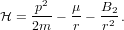(1)

Why a new routine

There are of course codes already available for this purpose; perhaps most notably the SWIFT routines. They are heavily tested and very reliable. However, I wanted to write my own routines, for a number of reasons.

• It was not straightforward for me to reach machine accuracy with SWIFT routines. In particular, on my laptop (AMD, x86-64) with GNU Fortran compiler, I explicitly had to use “-mfpmath=387” flag. Unless this flag is used, the code generated uses the double precision SSE instruction set. Unlike the 387 coprocessor instructions, SSE instructions do not store the temporary results in 80 bit precision. Seemingly this causes a small error (this was pointed out to me by Patricia Verrier). However, the error is consistent, so it adds up linearly in time, and decreasing the timestep makes things worse.
  I probably did not need machine precision in the first place, but it provides a peace of mind.
• I wanted something compact and in C, so I could play around with it more easily, parallelize the code, port it to GPUs etc.
• I wanted to see if continued fractions led to faster code (The speed improvement I obtained was negligible).
• Continued fractions are intriguing on their own. The functions we need to solve Kepler’s equation have surprisingly simple continued fraction expansions. Continued fractions allow infinite precision arithmetic (Gosper, 1972). Well, I do not know what to do about it at the moment, but it looks very interesting.

Please note that my experience with SWIFT routines is very limited. It is possible that one can make a few modifications to increase their accuracy while maintaining their reliability. I’d appreciate any feedback on this matter.

Solving Kepler’s equation

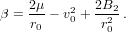
For simplicity let us initially assume B₂ = 0. Then the orbit is a Keplerian conic section. We start by calculating the quantities

(2)

where r₀ and v₀ are the initial position and velocity vectors, respectively. If β > 0, we have an elliptical orbit and can calculate the period

(3)

and the quantity

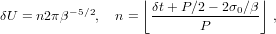(4)

where δt is the given time interval. This will be useful if δt > P, a situation that I do not encounter since I always choose timesteps much shorter than the period.

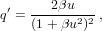
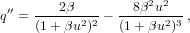
For our independent variable, we choose the initial value u = 0. The main loop consists of the following steps (prime denotes differentiation with respect to u):

(5)

(6)

(7)

(8)

(9)

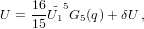(10)

(11)

(12)

(13)

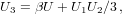(14)

(15)

(16)

(17)

(18)

(19)

(20)

(21)

(22)

(23)

(24)

(25)

(26)

Once the increment δu₃ or f is smaller than a preset tolerance, we exit the loop. The function G₅(x) is a special case of Gauss’s hypergeometric function: G₅(x) = ₂F₁(5,1;7∕2;x) (Abramowitz and Stegun, 1972, Ch. 15). The position and velocities are calculated by

(27)

(28)

(29)

(30)

(31)

(32)

This method of solution is almost identical to Shepperd’s. The only thing I did is to increase the order of the iteration by using Danby’s technique. In the actual implementation, if q > 1∕2 during iteration, or if convergence is not achieved after 12 iterations, we stop, and try to cover δt in two steps of δt∕2.

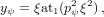
When B₂≠0, we need two modifications. In the following, I adopt the approach of Mikkola (1999); see that paper for generating functions etc. First note that in the plane of motion, we can transform to polar coordinates (r,θ) and write the Hamiltonian as

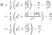(33)

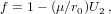
which is in Keplerian form. The first modification is

(34)

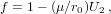
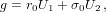
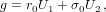
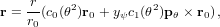
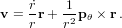
Furthermore, we cannot use f-g formulation directly, so at the end of the loop, we revert to a more general method, which is applicable for any motion with a radial force:

(35)

(36)

(37)

(38)

(39)

(40)

(41)

(42)

(43)

(44)

In this formulation c₀(x²) and c₁(x²) are Stumpff functions, and at₁(x²) is arctan(x)∕x. All these functions, and the function G₅(x) mentioned earlier, have simple continued fraction expansions. However, in my implementation, I only calculate G₅(x) by continued fraction expansion to keep things simple. An efficient way to do this is given by Shepperd (1985). For calculating c₀ and c₁ by continued fractions, probably the best way is to use the approach of Flanders and Frame (1987). The continued fraction for at₁(x) goes back to Lambert (1770) and Lagrange (1776) according to Olds (1963, Appendix II, formula 14):

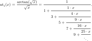(45)

The code

You can download the code from GitHub. The repository contains a few files. The most useful one is CF_kep_drift.c, which includes two routines. void drift_shep(double mu, double *r0, double *v0, double dt) solves Kepler’s equation for a particle with initial position r0, initial velocity v0, moving around a mass mu, over a time interval dt. The final positions and velocities are returned in r0 and v0. void drift_shep_pert(double mu, double B2, double *r0, double *v0, double dt) does the same but with perturbation B2. There is also a non-recursive version: drift_shep_nonrecurs(). This may be useful if you want to port the code to GPUs.

Kep_Drift_test.c is a small piece of code that I wrote to test my routines. It also has hooks for SWIFT routines, but I do not distribute them. If you download SWIFT, you can copy over the necessary files (listed in the Makefile), uncomment a few lines in the Makefile, change the definition of the macro DRIFT(mu, r, v) and compare the routines.

If there is some interest, I may post my comparison and other tests here.

Terms for using

This software is provided to help you get the job done. Hopefully to solve a problem, but possibly as a nice pastime. There are no restrictions whatsoever on the usage of this software. You can modify and adapt it to any use you see fit. However, I cannot be held responsible for any damage arising from using this software, including but not limited to wasting your time. Also, distributing the software, even parts of it as part of another software, is not usage. Such actions are governed by "Terms for copying and distribution", as indicated below.

I appreciate, but do not require, attribution. If you are unsure about what reference to use for attribution, feel free to ask. Note that, if you simply use this software to obtain some results to write a paper, you are not required to offer me co-authorship or such. Only if I provide extensive help to you for using the software, and hence I contribute significant amount of my time specifically for your project, I would like to be offered co-authorship. Do not let this to discourage you from asking questions, but please read the documentation (at least this page and possibly the references) before doing so.

In particular, feel free to port this code to GPUs. I also plan to do this at some point, but I think the code is already useful on its own.

Terms for copying and distribution

This software is copyright (c) 2008 by Atakan Gürkan, except where noted in the source files.

This program is free software; you can redistribute it and/or modify it under the terms of the GNU General Public License version 3 as published by the Free Software Foundation.

Note that I leave out the phrase "... or any later version", that is, you cannot merge this software with software under different versions of GPL. If you need to do this, please contact me and if the version you propose is reasonable for me, I will make an addition or exception to these terms.

This software is distributed in the hope that it will be useful, but WITHOUT ANY WARRANTY; without even the implied warranty of MERCHANTABILITY or FITNESS FOR A PARTICULAR PURPOSE. See the GNU General Public License for more details.

You should have received a copy of the GNU General Public License along with this program; if not, write to the Free Software Foundation, Inc., 59 Temple Place - Suite 330, Boston, MA 02111-1307, USA.

Parts of this software may be provided with licenses different from but compatible with GNU General Public License version 3. All such parts are clearly marked in the source code files. For those parts, you are free to use GNU General Public License version 3 or the particular license indicated in the source code.

Improvements and Bugfixes

If you make an improvement to this software, I would appreciate if you let me know about it. I also hope that you would allow me to further distribute your enhancements as part of this software, under the terms of this license. Note that, you do not need to transfer your copyright to me to make your improvements part of this software.

If you find an error in the formulae above, I really would like to hear about it. If there is an inconsistency between this text and the code, rely on the code. That is what I tested.

References

You can download a better typeset version of first few sections here (LaTeX source).

References

M. Abramowitz and I. A. Stegun. Handbook of Mathematical Functions. Dover, New York, 1972.
Richard H. Battin. An Introduction to the Mathematics and Methods of Astrodynamics. American Institute of Aeronautics and Astronautics, 1987.
J. M. A. Danby. Fundamentals of celestial mechanics, 2nd ed. Willman-Bell, Richmond, 1992.
Harley Flanders and J. Sutherland Frame. Algorithm of the bi-month: Elementary transcendental functions. The College Mathematics Journal, 18(5):417–421, 1987. ISSN 07468342. URL http://www.jstor.org/stable/2686970.
R. W. Gosper. Continued Fractions. MIT HAKMEM Artificial Intelligence Memo, no 239: item 101, 1972. http://www.inwap.com/pdp10/hbaker/hakmem/cf.html and http://keithbriggs.info/cfup.htm.
S. Mikkola. Efficient Symplectic Integration of Satellite Orbits. Celestial Mechanics and Dynamical Astronomy, 74:275–285, August 1999. doi: 10.1023/A:1008398121638.
Carl Douglas Olds. Continued Fractions. Random House, 1963.
S. W. Shepperd. Universal Keplerian state transition matrix. Celestial Mechanics, 35:129–144, February 1985.